Guest post: Why CO2 removal is not equal and opposite to reducing emissions
Application of instantaneous emissions and eliminations is an “idealised” way to run the experiment, but it is standard practice in environment science as the environment and carbon cycle reaction has actually been shown to be independent of the rate of emission or removal. Due to the fact that it is the minimum requiring that can be used for a temperature signal to be detectable, we utilize 100GtC as the smallest pulse size. This is even the case for a model like the one utilized in this study that leaves out atmospheric irregularity as there is still variability in the coupled ocean-sea ice-atmosphere system.
How about surface temperature level? It turns out that the response of temperature level to removals and emissions has less of this asymmetry. There is a 2% imbalance in temperature levels 100 years after a 200GtC emission or elimination, compared to 7% for atmospheric CO2..
There are reasons, however, to presume that the sign of the temperature level asymmetry will depend upon the climate design used to run the simulations. The temperature response to a CO2 emission and elimination is determined by the radiative impact of CO2 pointed out above, however likewise the uptake of heat by the ocean and climate feedbacks. The extent to which the mix of these procedures compensates the nonlinearity in the carbon cycle response most likely differs from design to model.
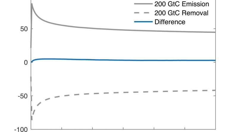
You can see this in the chart below, which shows an example of the simulated modification in atmospheric CO2 concentrations following the emission (strong grey line) or elimination (dashed grey line) of 200GtC. The blue line represents the difference in between the 2, which is somewhat positive– indicating that the increase in the climatic CO2 concentration following an emission is bigger than the decrease following an elimination of the very same magnitude.
Carbon cycle and environment actions vary widely in between models, and initial analysis of simulations with a set of complex Earth system models suggests that the magnitude of the carbon cycle and temperature asymmetry might be substantially larger than discovered in this research study..
For example, the CO2 fertilisation impact, by which plants produce more biomass under raised atmospheric CO2 concentration, fills at greater atmospheric CO2 levels. Also, the ability of the ocean to buffer excess CO2– which is key to the capability of the ocean to use up extra CO2 from the environment– reduces at higher climatic CO2 levels. An emission results in a different climatic CO2 concentration change than a removal of the same size because of these and other nonlinear processes.
In a new paper, published in Nature Climate Change, my coworkers and I show that the environment response to removals and emissions is really “asymmetrical”– that is, the carbon cycle and climate action to CO2 emissions is not equivalent and opposite to CO2 removals of the exact same magnitude.
While overall emissions and eliminations of as much as 500GtC as utilized in this study are constant with situations in the literature, emissions and eliminations in these scenarios take place concurrently and not in different CO2 emissions and removals “worlds”.
The requirement to reach zero carbon dioxide (CO2) emissions to stop the rise in worldwide average temperatures develops from the long time that CO2 remains in the atmosphere and the slow response time of the ocean..
This can be achieved by improving natural carbon “sinks” that get rid of CO2 from the atmosphere– for instance, by planting trees or bring back peatlands and mangrove forests. Other ways to remove CO2 from the atmosphere include catching CO2 from bioenergy plants or crafted techniques that catch CO2 straight from the atmosphere and shop it underground or in items.
Zickfeld, K. et al. (2021) Asymmetry in the climate– carbon cycle reaction to unfavorable and favorable CO2 emissions, Nature Climate Change, doi:10.1038/ s41558-021-01061-2.
In the real life.
But this assumption had not been tested, and– while most likely sensible for small emissions and removals– it seemed not likely to hold for larger emissions and eliminations due to the non-linear nature of the Earth system..
We chose to check our hypothesis utilizing a worldwide climate design of intermediate intricacy, with streamlined representation of some environment system parts and run at a coarser spatial resolution than models of full intricacy..
As a result of applying removals and emissions separately, the climatic CO2 concentration diverges more highly in our model simulations than it would in the real world, magnifying the asymmetry..
Emissions and removals.
Based upon these model simulations, we found that the modification in the concentration of CO2 in the atmosphere is unbalanced..
The figure listed below programs the global surface area air temperature reaction to 200GtC of emissions (solid grey line) and eliminations (rushed grey line). The distinction between the two (revealed by the blue line) exposes that the temperature level asymmetry is the opposite sign to the climatic CO2 concentration asymmetry: the temperature level boost following an emission is slightly smaller sized than the reduction following an elimination of the very same size..
The factor is that nonlinearities in the carbon cycle are compensated by another nonlinear procedure– that is, the impact of changes in climatic CO2 in the worlds radiation balance, which decreases at greater atmospheric CO2 levels. As an outcome, an increase in atmospheric CO2 has a smaller radiative impact than a CO2 reduction of the very same magnitude.
Sharelines from this story.
Modification in climatic CO2 concentration following a CO2 emission (strong grey line) and elimination (rushed grey line) of 200 GtC used from a climate state at balance with two times the pre-industrial climatic CO2 concentration. The CO2 fertilisation impact, by which plants produce more biomass under elevated atmospheric CO2 concentration, saturates at greater climatic CO2 levels. The ability of the ocean to buffer excess CO2– which is crucial to the ability of the ocean to take up extra CO2 from the atmosphere– lessens at greater atmospheric CO2 levels. Modification in internationally averaged surface area air temperature level following a CO2 emission (solid grey line) and elimination (rushed grey line) of 200GtC used from an environment state at balance with twice the pre-industrial climatic CO2 concentration. The temperature response to a CO2 emission and elimination is figured out by the radiative impact of CO2 mentioned above, but also the uptake of heat by the ocean and climate feedbacks.
Does the asymmetry discovered in this study have implications for how CO2 emissions and removals are stabilized in real-world settings?.
In conclusion, the findings of this research study suggest that stabilizing a CO2 emission with a CO2 removal might result in a different climate outcome than preventing the CO2 emission, however the magnitude of this result remains uncertain and calls for more metrology.
This asymmetry increases the more CO2 is given off or eliminated– from 3% for a 100GtC emission and elimination to 18% for a 500GtC emission and removal (relative to the atmospheric CO2 modification 100 years after the emission or elimination).
We forced the design with an immediate “pulse” of CO2 emissions and eliminations ranging from 100bn to 500bn tonnes (gigatonnes or GtC) of carbon, comparable to around 10 to 50 times current international annual CO2 emissions..
Modification in internationally averaged surface air temperature following a CO2 emission (solid grey line) and elimination (dashed grey line) of 200GtC used from an environment state at balance with two times the pre-industrial atmospheric CO2 concentration. The warming following an emission is somewhat smaller sized (blue line) than the cooling following a removal of the very same magnitude. Credit: Kirsten Zickfeld.
Modification in climatic CO2 concentration following a CO2 emission (solid grey line) and elimination (rushed grey line) of 200 GtC used from an environment state at equilibrium with two times the pre-industrial atmospheric CO2 concentration. The rise in the climatic CO2 concentration following an emission is larger than the decline following a removal of the very same magnitude (the blue line reveals the difference). Credit: Kirsten Zickfeld.
In the last few years, nations, companies and organizations around the globe have set “net-zero” emissions targets as part of efforts to deal with environment change.
The benefit of this class of designs is that they are quicker to run and, therefore, allow us to run more and longer simulations. The added advantage in this case is that the model does not represent climatic variability due to phenomena such as El Niño and La Niña. This makes it much easier to find a “signal” in how the Earth reacts to changing CO2.
If the atmospheric CO2 concentration is to stay the same, this finding indicates that additional CO2 removal is required to compensate for an emission. Or, in other words, that balancing a CO2 emission with a CO2 elimination of the very same size would lead to greater climatic CO2 than avoiding the CO2 emission in the very first location.
The asymmetry in the climatic CO2 concentration arises from differences in the method the land and ocean carbon sinks respond to emissions and eliminations. A number of crucial processes that determine the reaction of these sinks are not direct..
Temperature.
A presumption that is commonly made when balancing a CO2 emission with a CO2 elimination is that “one tonne in equates to one tonne out”– that is, that the behaviour of the environment system in action to eliminations and emissions is “in proportion”..
However how about the “net” aspect? The logic is that residual emissions of CO2– and other greenhouse gases that are extremely pricey or difficult to get rid of– can be balanced by removing CO2 straight from the atmosphere and storing it for the long term..